Using models
Models assign probabilities to events, and simulate new events.
Default parameters
When you create models, you can specify defaults for parameters:
m = hp.norm(loc=4, scale=2)
data = m.rvs(50)            # Uses loc=4, scale=2
m.pdf(data=data, scale=3)   # Uses loc=4, scale=3
Any unspecified parameter to methods like pdf is replaced by a default. Parameters always have defaults, even if you don’t specify any when making a model. For example, the defaults for loc and scale are 0 and 1. There are no ‘mandatory parameters’ to any model.
Unlike scipy.stats, passing defaults on initialization does not “freeze” parameters; see the fix and freeze methods for that[LINK].
You can also specify defaults via the params argument:
m = hp.norm(params=dict(loc=2))
which might help if some parameter names clash with argument names. but please don’t name your parameters ‘data’ or ‘quantiles’ anyway, it is confusing.
Default data
Besides parameters, you can also specify default data for use in the pdf, cdf, and diff_rate methods:
m = hp.norm(data=my_data, loc=4)
m.pdf()                     # Gives pdf(my_data | loc=4, scale=1)
and default quantiles for use in the ppf method:
m = hp.norm(quantiles=[0.3, 4, 2])
m.ppf()                     # Gives ppf([0.3, 4, 2])
Models may do some pre-computation on the provided default data. If you keep the data fixed while varying parameters (e.g. in fitting), providing the data as default can speed up computations. This:
m = some_model(data=...)
results = [m.pdf(params) for params in ...]
can be significantly faster than this:
m = some_model()
# Not so great
results = [m.pdf(data, params) for params in ...]
if the model is sufficiently complex.
Changing defaults
Models are immutable: they don’t change after they are created. You cannot change the default parameters or data on an existing model.
Instead, you can get new models with different defaults or data from old models, by calling them:
m = hp.norm(loc=1)
m2 = m(loc=2)              # m2 has default loc 3
m3 = m2(data=m2.rvs(10))   # m3 has default data
None of this causes m to change. Even if you do this:
m = m(scale=2) # new model assigned to m
you just make a new model and make the variable m point to it. The m2 and m3 models don’t change scale. The model m originally pointed to is also not modified, m just points to another model.
(The immutability of models is not enforced by python. If you monkey around with private methods or attribute assignments, sure, you can change models – but please don’t.)
Model methods
For all of the methods below, you can specify parameters through keyword arguments, or a params=dict(...) argument. Omitted parameters revert to their defaults.
The pdf method returns the probability density or mass function, depending on whether the model has continuous or discrete observables.
The cdf method returns the cumulative distribuition function, and ppf the inverse of the cdf. Note ppf does not take data, but quantiles (between 0 and 1) as its first argument.
Each model in hypney also has a rate. In settings where this is meaningful, it corresponds to the total number of expected events:
model = hp.norm()
model.rate()       # Gives 1.0
model.rate(loc=2)  # Gives 1.0
The default rate is 1. Most basic models have a rate parameter that determines the rate and does nothing else. Complex models may have a rate that depends on many or even all parameters; see e.g. cuts [TODO LINK].
You can simulate new data with the rvs method, which, like in scipy.stats, draws a specific number of events. Alternatively, the simulate method draws a dataset in which the number of events depends on the model’s rate:
model = hp.norm(rate=20)
data = model.rvs(50, scale=2)   # 50 events
data = model.simulate(loc=3)    # random number of events, mean 20
Models also have a mean and std method, which return the expected mean and standard deviation of an infinite dataset of observables. For complex models these may be very slow, or raise a NotImplementedError. For models with multiple observables their behaviour is currently undefined.
Vectorization
All model methods are vectorized over parameters:
>>> model = hp.norm()
>>> model.pdf(0, loc=[-1, 0, 1], scale=[1, 2, 3])
array([0.24197072, 0.19947114, 0.12579441])
>>> model.pdf([0, 1], loc=[-1, 0, 1], scale=[1, 2, 3])
array([[0.24197072, 0.05399097],
       [0.19947114, 0.17603266],
       [0.12579441, 0.13298076]])
You can specify parameters as arbitrary-shaped arrays/lists/tensors. The normal numpy broadcasting rules apply.
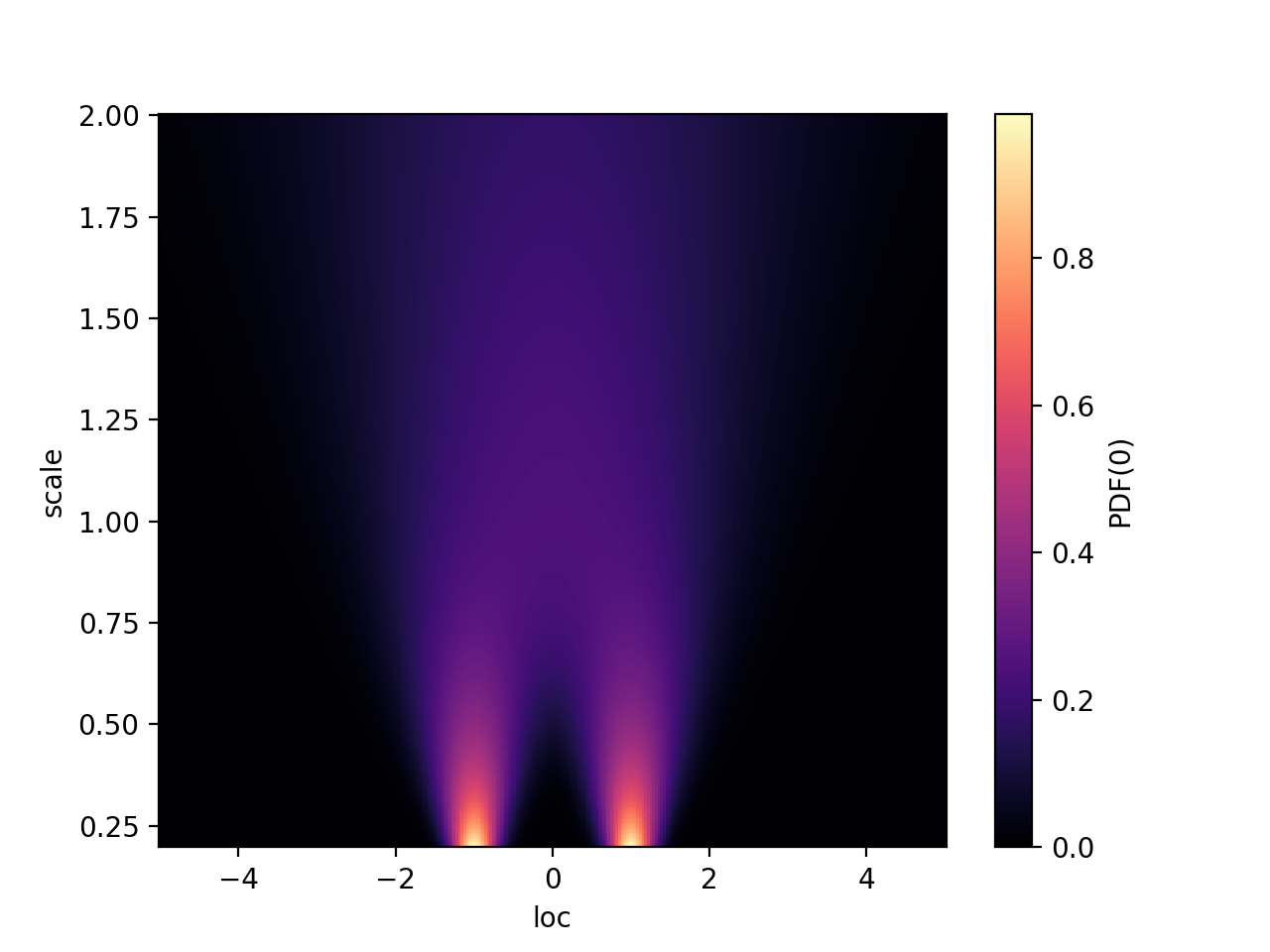
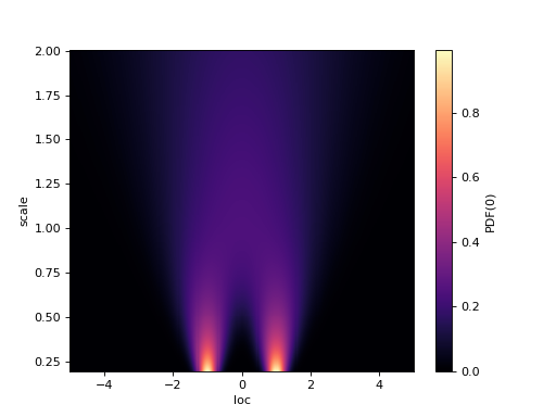
import hypney.all as hp
model = hp.mixture(
    hp.norm().shift(-1),
    hp.norm().shift(1),
    share=['loc', 'scale'])

loc = np.linspace(-5, 5, 300)
scale = np.linspace(0.2, 2, 300)
p = model.pdf(0, loc=loc[:,None], scale=scale[None,:])

plt.pcolormesh(loc, scale, p.T, shading='nearest', cmap=plt.cm.magma)
plt.xlabel("loc")
plt.ylabel("scale")
plt.colorbar(label='PDF(0)')
(Source code, png, hires.png, pdf)
Hypney always ‘batches’ over the entire dataset. You cannot specify different parameters for use on different events in a dataset.
Plotting
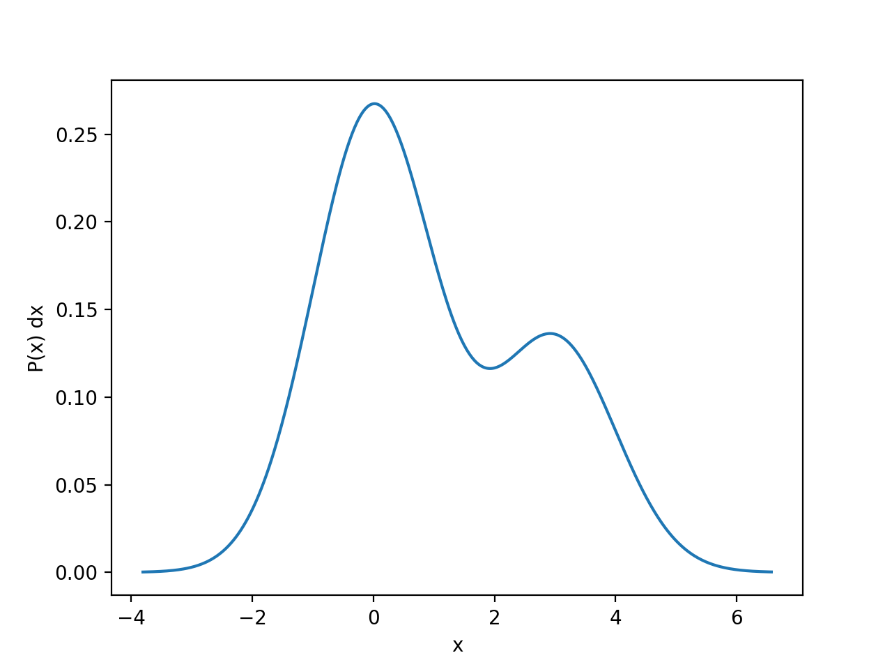
Hypney includes a small plotting helper to quickly inspect one-dimensional models. You can plot the PDF, CDF, and differential rate of a model:
m = hp.norm(rate=2) + hp.norm(loc=3)
m.plot_pdf()
plt.show()
(Source code, png, hires.png, pdf)

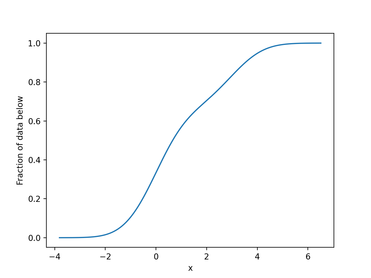
m.plot_cdf()
plt.show()
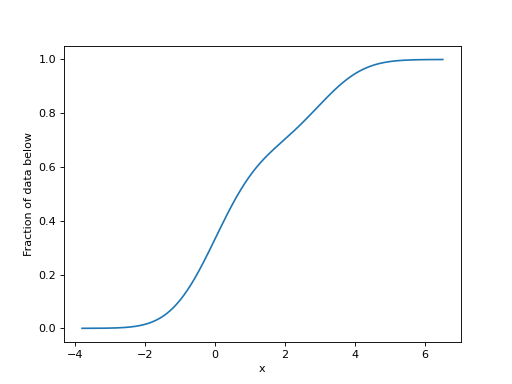
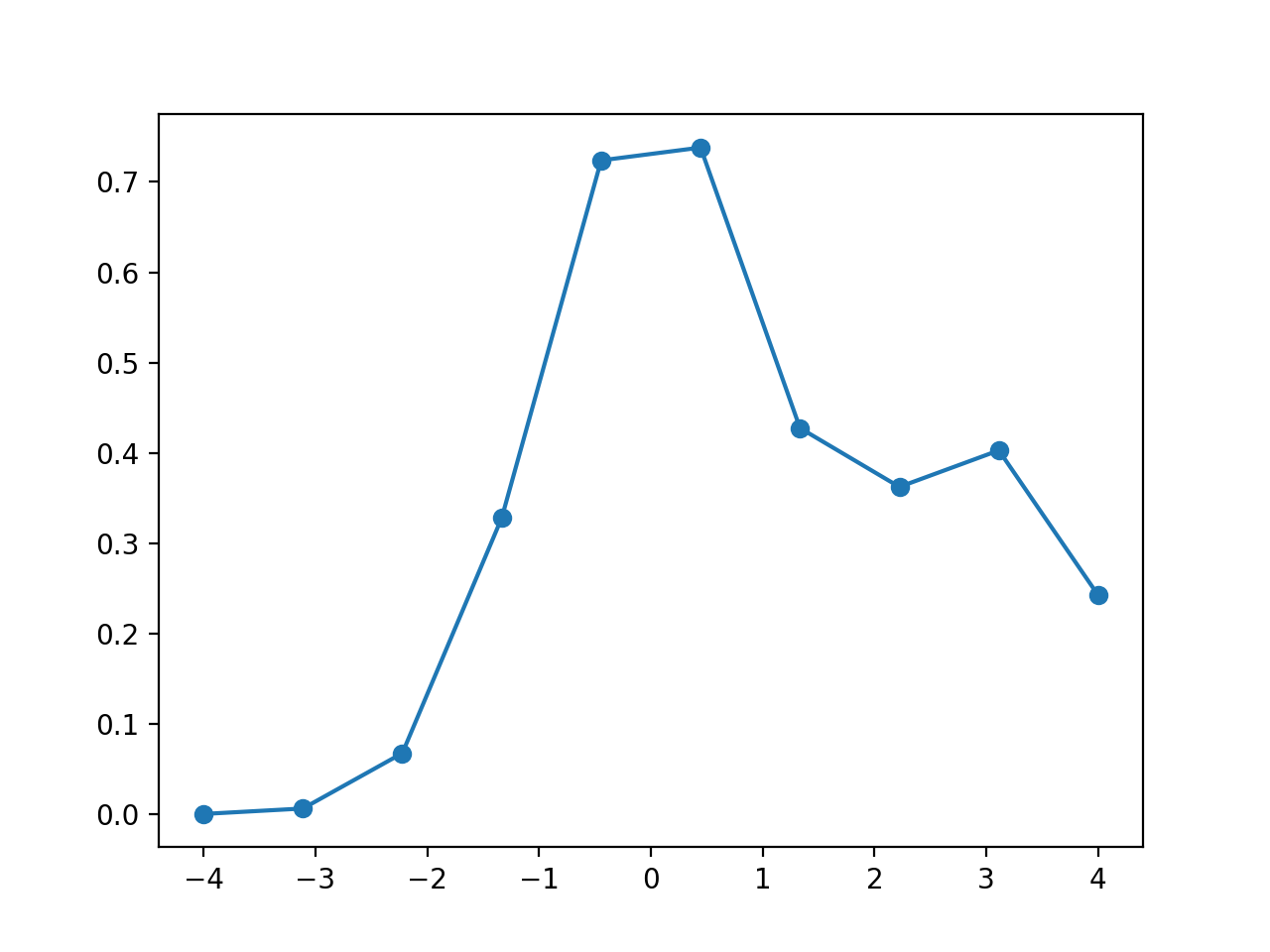
By default, hypney will guess upper and lower bounds to plot between. You can specify datapoints to plot over as the first argument. Other arguments are passed to plt.plot (or plt.hist for discrete observables). Passing auto_labels=False suppresses the default axis labels.
m.plot_diff_rate(np.linspace(-4, 4, 10), marker='o', auto_labels=False)
(Source code, png, hires.png, pdf)
