Building with models
Fixing parameters
The Model.fix method returns a model with fewer parameters than the original. You supply which parameters to fix to which values.
>>> hp.norm().defaults
{'rate': 1.0, 'loc': 0.0, 'scale': 1.0}
>>> hp.norm().fix(loc=2, rate=3)
{'scale': 1.0}
If you want a model with different defaults but the same parameters instead, just call the model as described in changing defaults [TODO link]:
The Model.fix_except method returns a model with all parameters but the ones you specify fixed to their defaults.
>>> hp.norm().fix_except('loc').defaults
{'loc': 0.0}
Reparametrize
The Model.reparametrize method returns a model with new parameters related to the old parameters. You supply a function giving a dictionary of old parameters from a dictionary of new parameters.
Cuts
The Model.cut method returns a new model for data thas has been restricted to an interval / rectangular region, after it was generated by the first model.
The new model takes the same parameters, which are simply passed on to the underlying model. For example, loc shifts the uncut model, while keeping the cut in place:
import hypney.all as hp

m = hp.norm()
m_cut = m.cut(-2, 2)

m.plot_pdf(label='Standard')
m_cut.plot_pdf(label='Cut')
m_cut(loc=1).plot_pdf(label='Cut, loc=1')
plt.legend()
(Source code, png, hires.png, pdf)
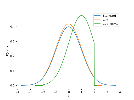
This shows the PDFs of a standard normal (blue), a standard normal cut to [-2, 2] (orange), and a normal with a mode of 1 cut to [-2, 2]. Notice the cut for the last model is still [-2, 2]; loc specifies the mean of the uncut model, it does not shift the cut model. To do that, see shifts and scales [TODO xref] below.
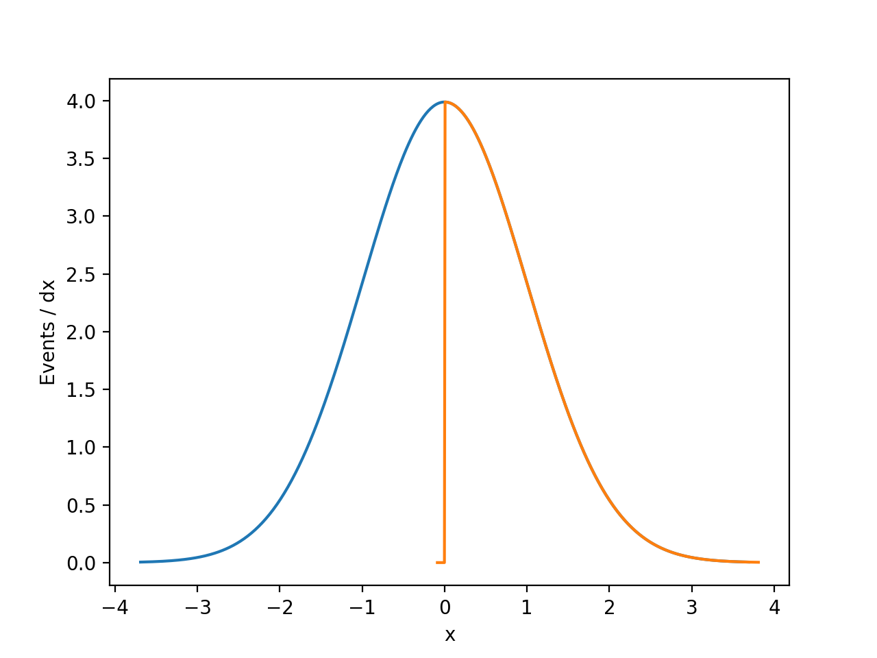
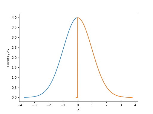
The total rate of a cut model is reduced by the cut’s efficiency. The differential rate is zero outside the cut, and unaffected inside the cut.
m = hp.norm(rate=10)
m_cut = m.cut(0, None)
assert m_cut.rate() == 5

m.plot_diff_rate()
m_cut.plot_diff_rate()
(Source code, png, hires.png, pdf)
Shift and scale
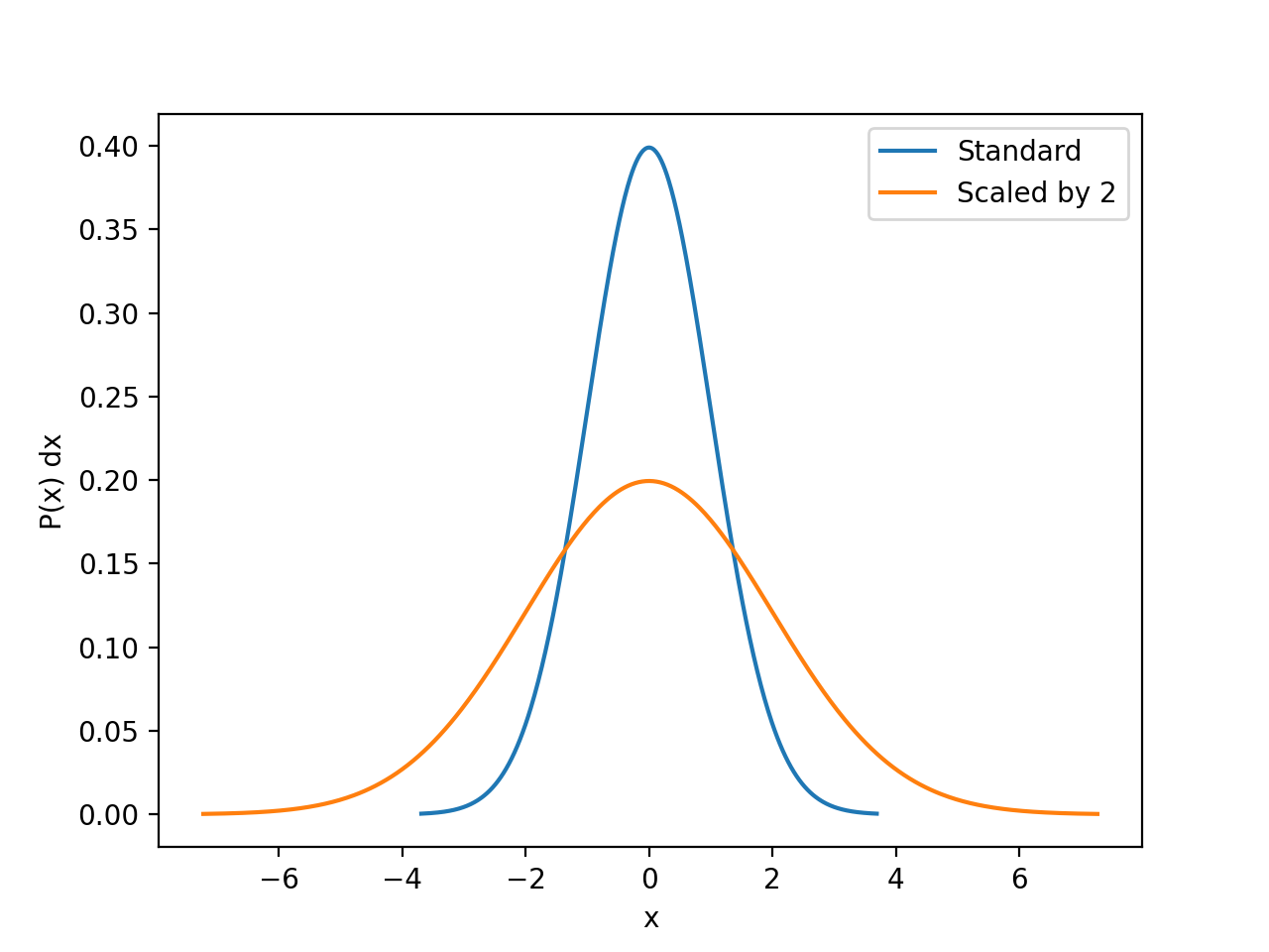
The Model.shift and Model.scale method return models for data that has been shifted (added to a constant) or scaled (multiplied by a constant) after being generated from the original model.
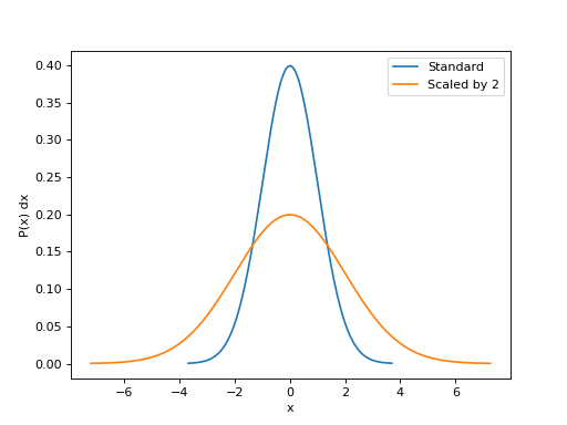
import hypney.all as hp
m_orig = hp.norm()
m_scaled = m_orig.scale(2)

m_orig.plot_pdf(label='Standard')
m_scaled.plot_pdf(label='Scaled by 2')
plt.legend()
(Source code, png, hires.png, pdf)
As with a cut model, the new model takes the same parameters, which are simply passed on to the underlying model. For example:
m_orig(loc=3).plot_pdf(label='Orig, loc=3')
m_scaled(loc=3).plot_pdf(label='Scaled by 2, loc=3')
plt.legend()
(Source code, png, hires.png, pdf)
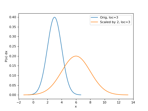
Setting m_scaled’s loc to 3 caused the model’s mean to shift to 6, not 3; as promised, loc controls the mean of the model before the factor 2 scaling.
Sums / mixtures
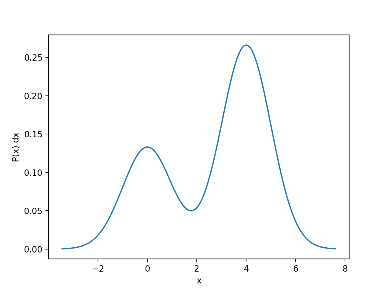
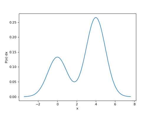
You can create mixture models with the + operator. This produces a model for data created from multiple models joined/concatenated together. The rate of the summed model is the sum of the original models’ rates.
m0 = hp.norm()
m1 = hp.norm(loc=4, rate=2)

m_sum = m0 + m1
m_sum.plot_pdf()
assert m_sum.rate() == 3
(Source code, png, hires.png, pdf)
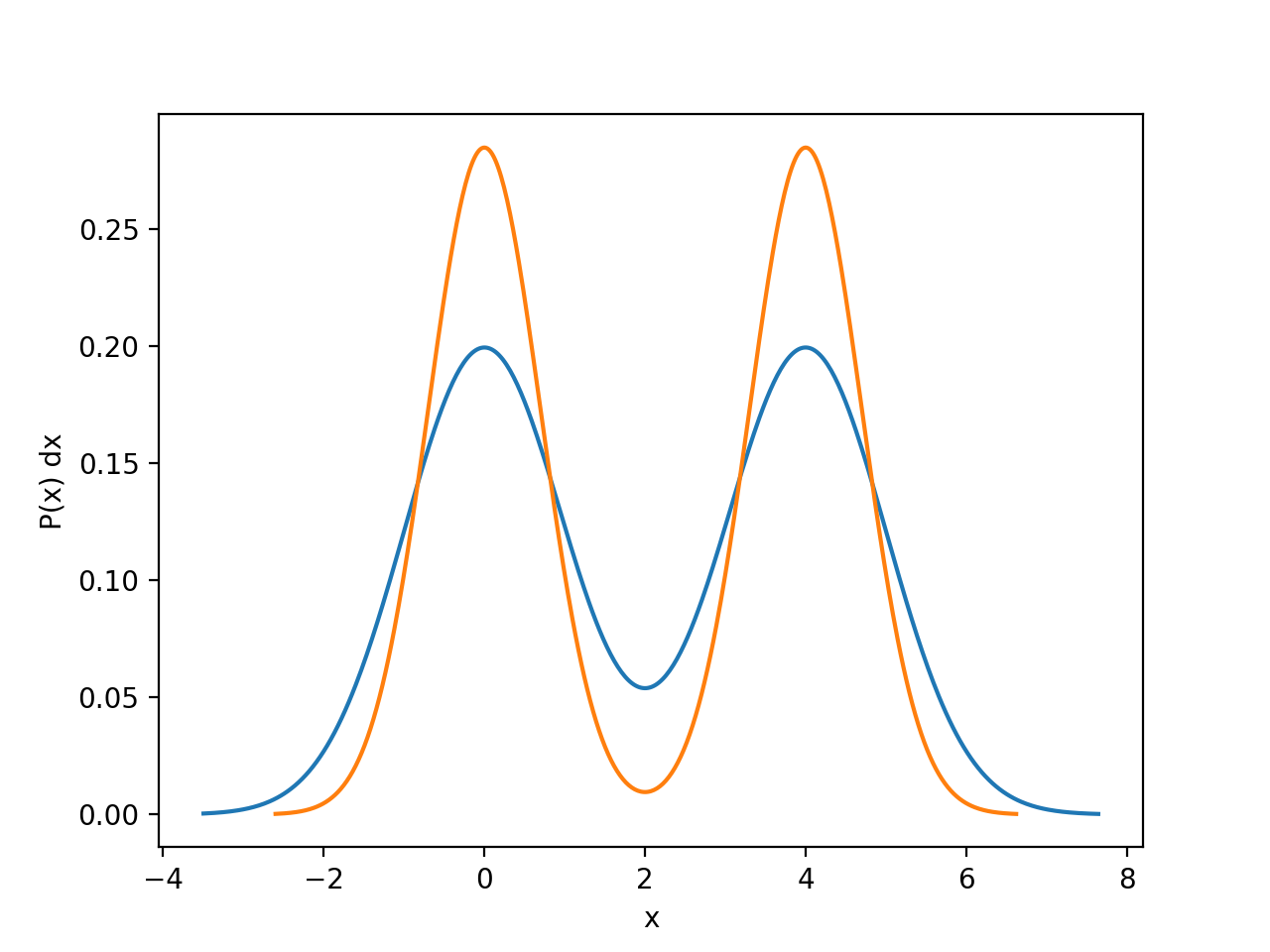
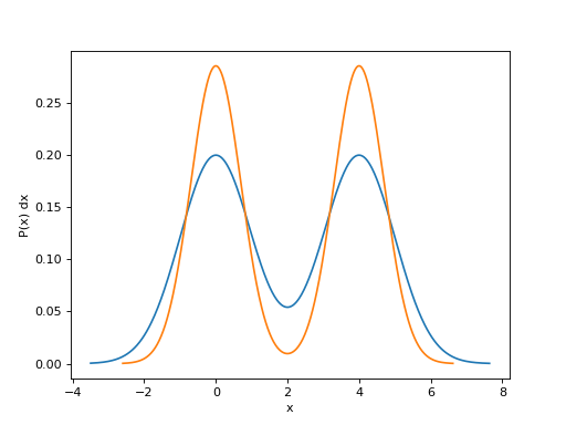
You can also use Model.mix_with(*other_models) and hypney.models.mixture(*models) instead of the power operator. This gives additional options, such as the ability to share parameters with the same name:
m_shared = hp.mixture(m0, m1, share=['scale', 'rate'])
m_shared.plot_pdf()
m_shared(scale=0.7).plot_pdf()
(Source code, png, hires.png, pdf)
Unshared parameters with clashing name are renamed to {model_name}_{param_name}. If the models have no name, “m{I}” is used, where {I} is the index of the model in the mixture.
>>> m_sum.param_names
('m0_rate', 'm0_loc', 'm0_scale', 'm1_rate', 'm1_loc', 'm1_scale')
>>> m_shared.param_names
('rate', 'm0_loc', 'scale', 'm1_loc')
Tensor Products
The power operator ** creates a model for multiple observables on the same events (e.g. time and energy) from models for the individual observables. This is known as a ‘tensor product’ of distributions.
For example, this generates a two-dimensional model for data with a normally distributed and a uniformly distributed observable:
m_2d = hp.norm() ** hp.uniform()

data = m_2d.rvs(1_000)
plt.scatter(data[:,0], data[:,1], c=m_2d.pdf(data), vmin=0)
plt.colorbar(label='PDF')
You can also use Model.tensor_with(*other_models) and hypney.models.tensor_product(*models) instead of the power operator.